|
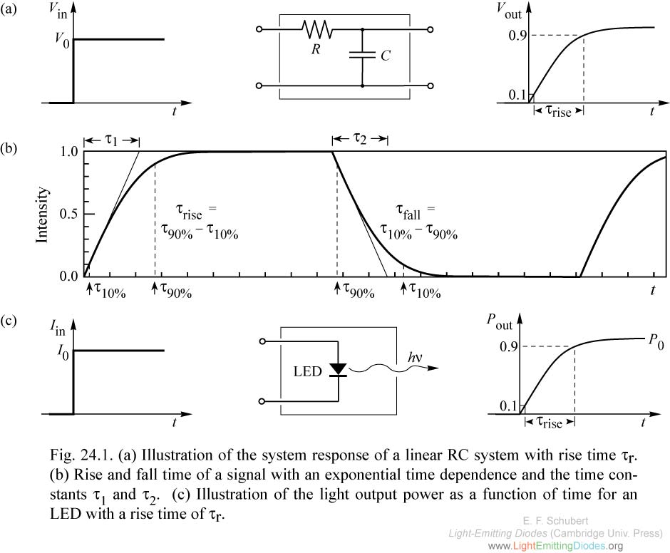
Fig. 24.1. (a) Illustration of the system response of a linear RC system with rise time tr. (b) Rise and fall time of a signal with an exponential time dependence and the time constants t1 and t2. (c) Illustration of the light output power as a function of time for an LED with a rise time of tau r.
|
|
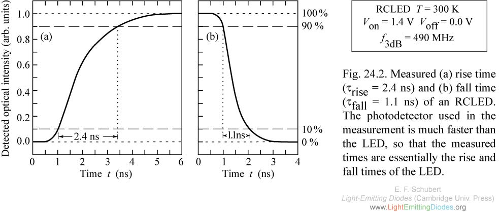
Fig. 24.2. Measured (a) rise time (tau rise = 2.4 ns) and (b) fall time (tau fall = 1.1 ns) of an RCLED. The photodetector used in the measurement is much faster than the LED, so that the measured times are essentially the rise and fall times of the LED.
|

|
Fig. 24.3. (a) Cross section micrograph of an AlGaAs LED grown on a transparent GaP substrate. (b) Electroluminescence originating from a current-injected region located under a stripe-shaped contact viewed through the transparent GaP substrate (after Woodall et al., 1972).
|
|
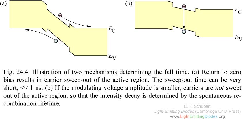
Fig. 24.4. Illustration of two mechanisms determining the fall time. (a) Return to zero bias results in carrier sweep-out of the active region. The sweep-out time can be very short, << 1 ns. (b) If the modulating voltage amplitude is smaller, carriers are not swept out of the active region, so that the intensity decay is determined by the spontaneous recombination lifetime.
|
|
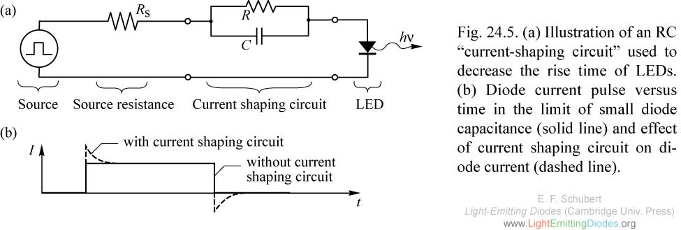
Fig. 24.5. (a) Illustration of an RC “current-shaping circuit” used to decrease the rise time of LEDs. (b) Diode current pulse versus time in the limit of small diode capacitance (solid line) and effect of current shaping circuit on diode current (dashed line).
|
|
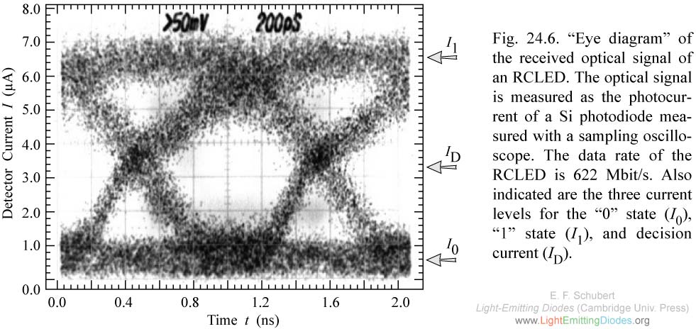
Fig. 24.6. “Eye diagram” of the received optical signal of an RCLED. The optical signal is measured as the photocurrent of a Si photodiode measured with a sampling oscilloscope. The data rate of the RCLED is 622 Mbit/s.
|
|
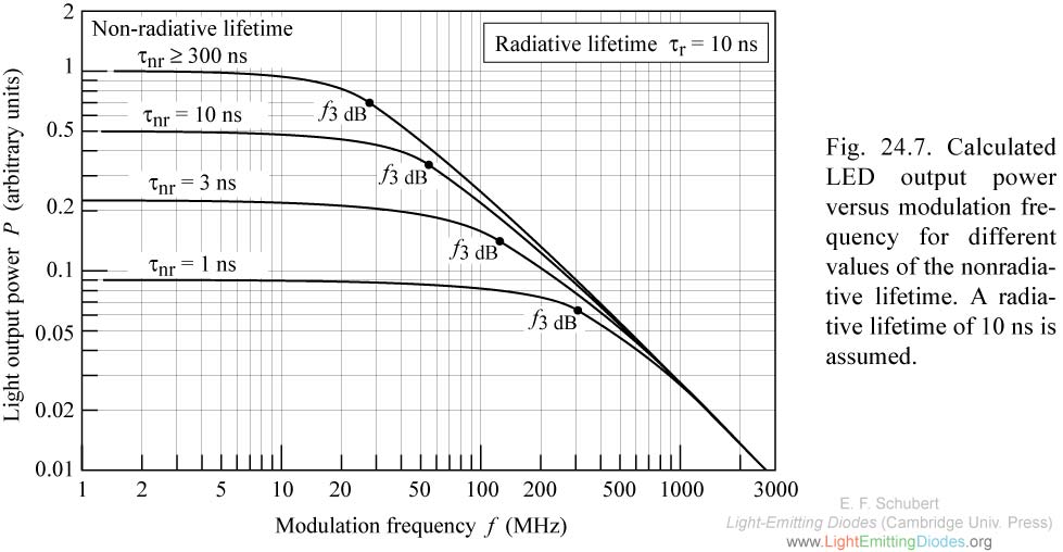
Fig. 24.7. Calculated LED output power versus modulation frequency for different values of the nonradiative lifetime. A radiative lifetime of 10 ns is assumed.
|